Lab 7: Processor Simulation with Sniper

Outline#

In this week’s lab you will:

Learn about the Sniper multicore simulator
Learn how to simulate programs and program traces
Learn how to specify CPU parameters in Sniper
Quantitatively analyse timing information from Sniper
Learn about and quantify processor energy consumption

Building Sniper#

The first step is to fork and clone the Sniper simulator repository from Gitlab. Once you have a local copy of the repository, you can build Sniper using the command make -j`nproc` from inside the sniper directory. This takes a while so continue reading the next section while you wait for the compilation to finish.

We have set up the lab machines with all the required dependencies to build and run Sniper. If you want to set it up on your laptop or another machine,you can find instructions on the Sniper website. Also note that you can also get remote access to lab machines via SSH using partch.

The Sniper Simulator#

Sniper is a state-of-the-art CPU simulator that can quickly and accurately simuate x86 processors. Unlike the first half of the course, Sniper does not precisely model all the timing and digital logic inside the CPU. Instead, it uses a technique called (interval simulation)[]. Sniper analyses a stream of instructions and breaks down the execution time into (1) time during which the processor is smoothly executing instructions and (2) time wasted due to certain miss events. The miss events include branch mispredictions, cache misses, and so on. The miss events block the processor from smoothly executing instructions. Sniper then uses analytical modeling of miss events to determine the number of cycles each miss event takes to resolve and then moves on to the next instruction. Using this technique Sniper can quickly simulate complex interactions between the various components of a processor without actually modelling the time that the CPU is blocked. Sniper is hence called a cycle-level simulator. Other simulators (e.g., Gem5) are much slower as they faithfuly model a processor on a cycle-by-cycle basis using event loops. They are called cycle-accurate simulators.

Sniper Overview

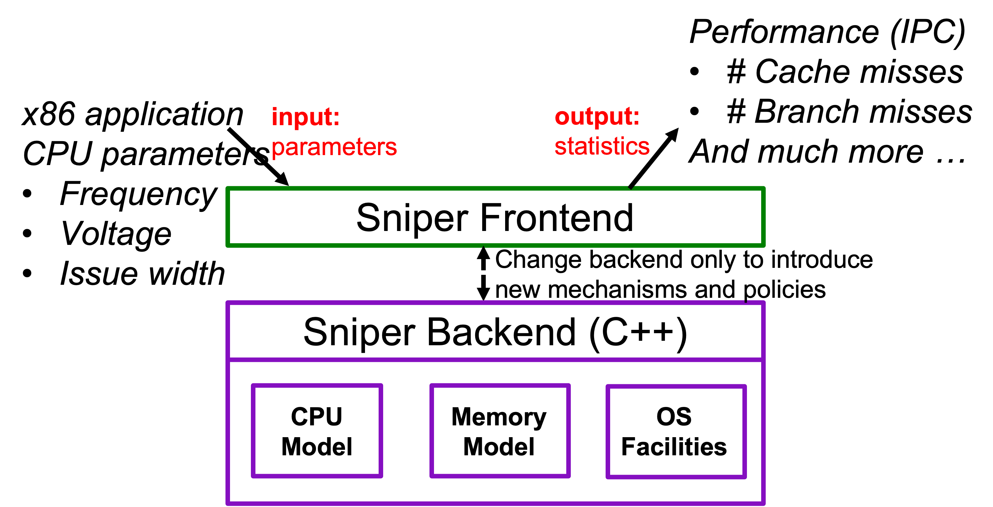
Sniper tracks and reports various metrics, such as, cycles per instruction (CPI), cache misses, memory accesess, reads and write count, and a lot more. It also includes tools that can be used to analyse and visualise this data, including bottleneck analysis. Using this data we can learn how a processor performs under various workloads and tune parameters to improve its performance. This way we do not need to fabricate the processor first (saving millions of dollars) to measure its performance on workloads of interest. In this lab, we will focus on two pieces of data: the CPI stack and the power/energy consumption.

The backend of Sniper implements the various subsytems of a processor. This backend is written in C++. We will go into more detail of how the backend works and modify it in a future tutorial.

Sniper is incredibly powerful and we will not have time to talk about all its capabilities. If you are interested in reading further you can find more information on the Sniper website.

Running Sniper#

Run Sniper with the following command from inside the sniper directory: ./run-sniper -- /bin/ls. You should see the following ouptut. It takes a few seconds so be patient:

[SNIPER] Warning: Unable to use physical addresses for shared memory simulation.
[SNIPER] Start
[RECORD-TRACE] Using the Pin frontend (sift/recorder)
[SNIPER] --------------------------------------------------------------------------------
[SNIPER] Sniper using SIFT/trace-driven frontend
[SNIPER] Running full application in DETAILED mode
[SNIPER] --------------------------------------------------------------------------------
[SNIPER] Enabling performance models
[SNIPER] Setting instrumentation mode to DETAILED
CHANGELOG      decoder_lib  LICENSE           NOTICE     power.xml     riscv              sim.stdout
common         docker       LICENSE.interval  pin        python_kit    run-sniper         standalone
COMPILATION    Doxyfile     Makefile          pin_kit    README        scripts            test
config         frontend     Makefile.config   power.png  README.arm64  sift               tools
CONTRIBUTORS   include      mbuild            power.py   README.riscv  sim.cfg            xed
cpi-stack.png  lib          mcpat             power.txt  record-trace  sim.stats.sqlite3  xed_kit
[TRACE:0] -- DONE --
[SNIPER] Disabling performance models
[SNIPER] Leaving ROI after 4.26 seconds
[SNIPER] Simulated 0.6M instructions, 0.9M cycles, 0.68 IPC
[SNIPER] Simulation speed 151.0 KIPS (151.0 KIPS / target core - 6622.5ns/instr)
[SNIPER] Setting instrumentation mode to FAST_FORWARD
[SNIPER] End
[SNIPER] Elapsed time: 8.51 seconds

This command ran the program /bin/ls in Sniper. In fact, you can see the output of ls in the middle of Sniper’s output. The last few lines also give us some interesting statistics; Sniper simulated 0.6 million instructions in 0.9 million cycles which gives 0.68 instructions per cycle (IPC). You can also calcuate the cycles per instruction (CPI) by taking the reciprocal of this number.

You should see four new files:

sim.cfg - this contains the CPU parameters used in the simulation.
sim.info - this contains information about the simulator and command line parameters that were used to run the simulation.
sim.out - this contains statistics about the program and the performance of various components of the processor.
sim.stats.sqlite3 - this is a database file that contains all the data and metrics gathered during simulation. It is read and processed by the various analysis tools included with Sniper.

Have a look through these files and try to answer the following questions:

How many levels of cache were used?
What was the associativity of the l1 cache?
What replacement policy did each cache use?
What is the dispatch width of the processor?
How many cycles delay does a branch misprediction cause?
How many branch instructions were executed?
What is the miss rate of each of the caches?

SIFT traces#

Real-world programs consist of billions of instructions, and simulating entire programs is extremely time-consuming. To track the different metrics, Sniper needs to track each instruction’s side effects. For example, it needs to know the memory address of a load/store instruction to determine a cache hit or a miss. Similarly, it needs to track flags to determine a branch direction. This cost can become prohibitively expensive, especially at the testing scale that processor designers do. To get around this, Sniper uses program traces called SIFT traces. SIFT is a Sniper-specific format that records a trace of a subset of instructions in a large application, so instead of calculating the result of each instruction, Sniper can just read it from the trace. This process significantly increases the speed of the simulation and enables rapid prototyping. This way, a representative part of the benchmark needs to be recorded only once and can be reused for all future timing simulations as we evaluate different microarchitecture configurations.

We provide you with SIFT traces of 11 SPEC benchmarks. Each of these traces run approximatly 10 million instructions. Do an upstream pull of the lab repository to obtain the traces.

In next week’s tutorial, we will look at a more comprehensive quantitative analysis using all traces, but for this week, we ask you to pick one or two traces and focus on analysing their behavior by changing various processor parameters as described in the following exercises.

To run Sniper on a trace use the --trace flag e.g. ./run-sniper --traces=trace-name.

Specifying Processor Parameters#

To specify processor parameters in a simulation we have two options. First, we can set each parameter individually using the -g flag. For example, you could increase the branch misprediction penalty with ./run-sniper -g perf_model/branch_predictor/mispredict_penalty=16 --traces=trace-name. The second option is to use a configuration file found in the config/ directory in the sniper repository using the -c flag to set a number of parameters at once. Sniper comes with a couple predefined microarchitechtures. To run a simulation of a core using Intel’s Nehalem microarchitecture you would run the command ./run-sniper -c nehalem --traces=trace-name. Have a look at the file config/nehalem.cfg to see the parameters used. You can also use multiple of each of these flags and mix and match to test various configurations, for example:

./run-sniper -c nehalem -g perf_model/branch_predictor/mispredict_penalty=16 -g perf_model/core/frequency=2 --traces=trace-name

This command will use the nehalem configuration file but override the mispredict penalty and the frequency of processor with the specified values.

Another useful flag is -d. You might have noticed that the output files from a simulation always end up in the current directory, overriding any previous outputs. This isn’t super helpful when you want to compare two different simulation outputs. -d allows you to tell Sniper where to put the output files. Appending -d ~/sim_output will put the output files in the directory sim_output in your home directory.

CPI Stacks#

Run the Sniper on your chosen SIFT trace with the following command:

./run-sniper -c gainestown -c rob --traces=trace-name

Find out the dispatch width of the processor and use that to calculate the ideal CPI of the processor (hint: ideally the processor should be issuing, dispatching and retiring that number of instructions each cycle). You’ll quickly realise that the actual CPI is higher than that. Remember, we want a low CPI, this is the average number of cycles each instruction took to execute. On superscalar processors we want this to be below one meaning we are executing more than one instruction each cycle.

Why is the CPI higher than theoretically possible? What factors could contribute to this. Think about this and discuss it with someone before continuing.

We can use a CPI stack to gain insight into the delays caused by various miss events. Sniper includes a tool to generate CPI stacks from the output of a simulation. Run the command ./tools/cpistack.py (use the -d flag to specify a directory if the simulation output data is not in your current directory). You should get something that looks like the following (the actual numbers may differ depending on which trace you have used):

                      CPI       Time
base                 0.24     59.84%
rs_full              0.03      8.45%
branch               0.02      4.50%
mem-l1d              0.07     17.45%
mem-l2               0.02      3.90%
mem-dram             0.02      5.05%
other                0.00      0.80%

total                0.41    100.00%

You can visualize the bottlenecks by plotting the above data as a CPI stack.

CPI Stack

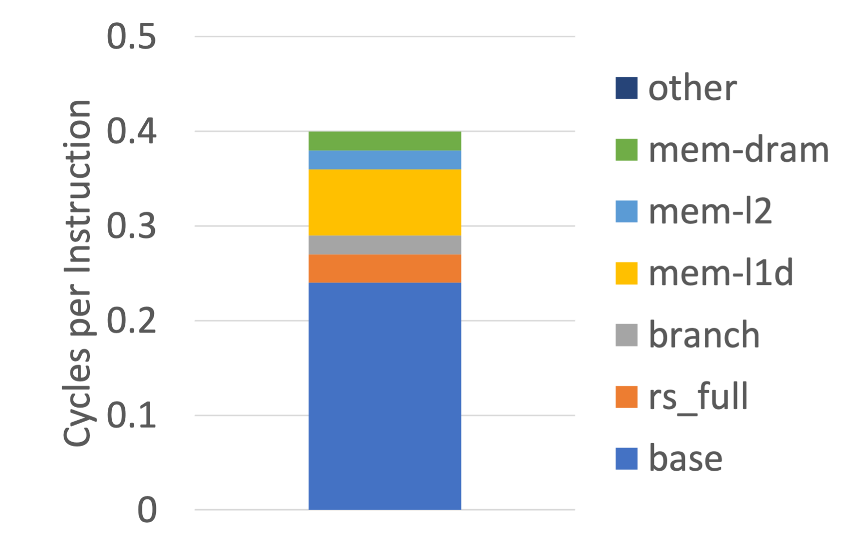
The base component represents the inherent cycle cost of each instruction. If a processor was running smoothly with no miss events this components would make up 100% of the CPI stack. All other components come from miss events. The values in the CPI column represent the number of cycles where the processor stalled due to that miss event averaged accross all instructions. Consider a single issue processor executing 10 instructions and in the middle there was a l1 cache miss that caused a 2 cycle delay. This would mean the total execution time was 12 cycles for a CPI of 1.2. The stack would have a base component of 1 and a mem-l1 component of 0.2.

The CPI stack gives us insight into what prevents processors from continuously executing instructions and how each type of miss event contributes to processor stalls. Run the simulation, modifying the dispatch width to see how this impacts the CPI stack. What is the ideal dispatch width for a processor running your chosen benchmark?

Identify the largest component of the CPI stack for your chosen benchmark. Have a look through the various parameters that are available (You can do this by looking at the various config files or looking at the contents of sim.cfg), which parameters would you optimise to reduce this component? It might be helpful to look at the CPI stacks of a couple different traces to get a more comprehensive picture.

Interpreting the Base Component#

It is crucial to interpret the base component of the CPI stack correctly to find the processor’s optimal dispatch width for a specific application. Consider a processor with a dispatch width (D) of two which means that under ideal circumstances, the processor can dispatch (or start) two instructions per cycle. Conversely, the minimum number of cycles we need to execute N instructions is N divided by D. If we have two instructions to execute, we at least need one cycle. For four instructions, we need a minimum of two cycles. Therefore, the base component is approximated as one divided by D. (If D is equal to four, then each instruction at least requires 0.25 cycles.) In reality, the smooth flowing and dispatching of instructions is impacted by true dependences. The actual dispatch bandwidth is typically less than the ideal width (two in this example).

Let’s look at an example. Suppose an application A running on a processor with a dispatch width of two has a base component equal to one. First, it means that the processor is not operating at its ideal dispatch capacity. We could reduce the base component by half. The processor cannot find sufficient ILP or independent instructions to execute with a dispatch width of two. Maybe it is worth increasing the dispatch width from two to four (hypothesis). Or perhaps not (after all the processor is not exploiting the dispatch capacity to its full potential!). That’s why we need a simulator to quickly verify a hypothesis.

Other Components#

First, at a high level, the memory systems consists of n levels of the cache hierarchy beyond which lies the physical memory or the main memory. The predominant main memory technology in use today is Dynamic Random Access Memory (DRAM). In typical high-performance processors today, n=3, i.e., three levels of the cache hierarchy. Mobile processors usually have a 2-level cache hierarchy. Also, the level-1 cache (L1) is divided into an instruction (L1-I) and data (L1-D) cache.

The CPI stack components you see include:

mem-l1d: This is the # cycles spent waiting for a response from the L1-D cache, i.e., L1-D hit cycles. If data is not present in the L1-D cache, the request is sent to level-2 (L2) cache which is bigger.
mem-l2: # cycles wasted due to waiting for L2 cache, i.e., L2 hit time.
mem-l3: A miss in L2 reaches L3. This component is the # cycles wasted (or # cycles the processor waited) for a response from L3 cache.
mem-dram: # cycles the processor waits for a response from DRAM.
branch: # cycles the processor spends in recovering from mispredicted branches. It involves flushing the pipeline of the speculative state (including instructions in flight) and setting the PC to execute instructions from the correct path.
rs-full: the time dispatching of new instructions is blocked because there are no more free entries in the scheduling window (or reservation stations).
ifetch: Typically, processors fetch 64 bytes from the L1-I cache which delivers enough instructions every cycle to keep the processor busy. But for very irregular code and where the branch predictor is unable to help with predicting the fetch targets accurately, the instruction fetch latency appears on the critical path. This is especially true if the processor needs to wait for instructions from main memory which has a latency of a few 100 cycles. No instructions, no progress.

Processor Power#

To understand the power consumption of a processor, you first need to understand a little bit of how modern MOS transistors and how logic gates are built. Logic gates are structured in such a way that when they are in a stable state (i.e., their inputs are not changing) they consume no power (this is not quite true but we will discuss this later). Only when transistors in the logic gate switch from one state to another (zero to one or vice-versa) does current flow and power is dissipated. This means that the power draw from a processor is not continuous. It rather spikes each clock cycle when transistors change state. This non-continuous power draw is called the dynamic power of a processor and is calculated as follows $P_{d y n a m i c} = \frac{1}{2} A C V^{2} N F$ .

$V$ is the voltage of the processor.
$C$ is the capacitance of a transistor. This capacitance represents residual charges that buildup and are discharged. Its quantity is determined by the transistor technology and fanout (the number of transistors connected to an output).
$N$ is the number of transistors in the processor.
$F$ is the frequency of the processor. As the frequency increases transistors switch more often and hence consume more power.
$A$ is the activity factor. Not every transistor will switch every cycle. This is a scalar value between 0 and 1 representing the average number of transistors that switch each cycle.

Given these parameters we can calculate the dynamic power of a processor. Because this is a dynamic power draw it can be reported as either peak (the maximum power draw at any one time) or average. Consider the uses of these two quantities: when would you care about each of them?

We said above that gates only consume power when they are switching, but this is an assumption and it isn’t completely true. In reality, a small amount of current is always leaking across transistors, even when they are not conducting. The power this phenomenon drains is called the static power and is calculated as follows $P_{s t a t i c} = V I_{l e a k}$ where $I_{l e a k}$ is the current that leaks through the transistors in a processor. Historically, dynamic power is much greater than static power, however as transistors have become smaller, the leakage current has increased. In fact, static power is the main culprit behind stagnated frequencies since 2005.

Given the static and dynamic power, we can calculate the total power consumption of a processor as $P_{t o t a l} = P_{d y n a m i c} + P_{s t a t i c}$ . We can also therefore calculate the total energy consumed by a processor as the product of power and execution time, $E = P_{t o t a l} X t$ where $t$ is the execution time.

The derivations of the formula presented above are interesting but not directly relevant to the course. If you are interested, you can find a lot of good content online (the physics isn’t especially complicated).

Both the power and energy are important quantities to consider. The total power of a processor dictates the cooling requirements and packaging of a processor while the energy informs us about the overall efficiency of the processor.

Now think about what would happen if you decreased the frequency of a CPU. More specifically, how would this affect its power consumption and the energy consumed by the processor? The voltage of a CPU is also dependant on the frequency. For the processor to run at a higher frequency, the voltage needs to be increased. Given this information what impacts do you think changing the frequency has?

Consider the two processors below executing the same workload. Which is more efficient?

	Power (Watts)	Execution Time (seconds)
Processor A	100	100
Processor B	60	150

There are two more metrics that are important. The energy delay product ( $E D P$ ) takes into account that decreasing the energy consumption can increase the execution time. The product of energy and delay (or execution time) is important here to balance the saved energy with the longer time it takes to compute. (Without EDP, someone can report reduced energy consumption by decreasing power too much at the expense of really poor performance.) There is also the $E D^{2} P$ which again biases the result further to a lower execution time. Consider the two processors above with these metrics? Which one is better now?

Sniper allows you to modify the frequency and the voltage of the processor it is simulating. The frequency parameter is perf_model/core/frequency in GHz and the voltage parameter is power/vdd in V. Sniper also includes a tool to calculate the power and energy consumption of the different components of a processor called McPAT (originally from HP Labs). To run McPAT use ./tools/mcpat.py (as with the CPI stacks, use -d to specify the directory of the simulation output). You should get something that looks like the following:

                   Power     Energy    Energy %
core-core         1.87 W     0.67 mJ     11.23%
core-ifetch       0.58 W     0.21 mJ      3.52%
core-alu          0.29 W     0.11 mJ      1.75%
core-int          0.50 W     0.18 mJ      3.01%
core-fp           0.74 W     0.27 mJ      4.47%
core-mem          0.51 W     0.18 mJ      3.07%
core-other        1.03 W     0.37 mJ      6.19%
icache            0.45 W     0.16 mJ      2.70%
dcache            1.16 W     0.42 mJ      6.96%
l2                0.43 W     0.15 mJ      2.57%
l3                3.39 W     1.22 mJ     20.41%
dram              5.64 W     2.04 mJ     33.96%
other             0.03 W     9.36 uJ      0.16%

core              5.53 W     1.99 mJ     33.24%
cache             5.42 W     1.96 mJ     32.64%
total            16.62 W     5.99 mJ    100.00%

You can see the power and energy consumption of each component of the CPU.

Try running Sniper with the following voltage and frequency configurations, and then run McPAT to see how they impact the power and energy consumption.

Voltage (V)	Frequency (GHz)
0.79	1.50
1.07	4.00

Look at the McPAT results and CPI stacks of both configurations. What differences do you notice?

Pick a specific trace and analyse the impact on performance, power, and energy of changing various processor parameters. Manipulate both CPU and memory-related parameters even if you do not yet have a full understanding of the memory system. Observe the CPI stacks and the McPAT output.

Wrapping Up#

Hopefully you have gotten a good indication of the types of analyses that can be performed using the Sniper simulator. If you have time keep experimenting with different parameters, try different traces. There are many more features that we didn’t cover in today’s lab. If you are interested in learning more have a look at the Sniper website. Next week you will perform more in-depth quantitative analysis using the tools you learned about today and the week after that we will delve into the backend of Sniper.