so far: synthesisers

creating sound from scratch with basic waveforms/shapes

now: recordings

finding sounds from the real world, recording and manipulating

first explored in the analogue era, e.g., Études de bruits (1948)

Musique Concrète

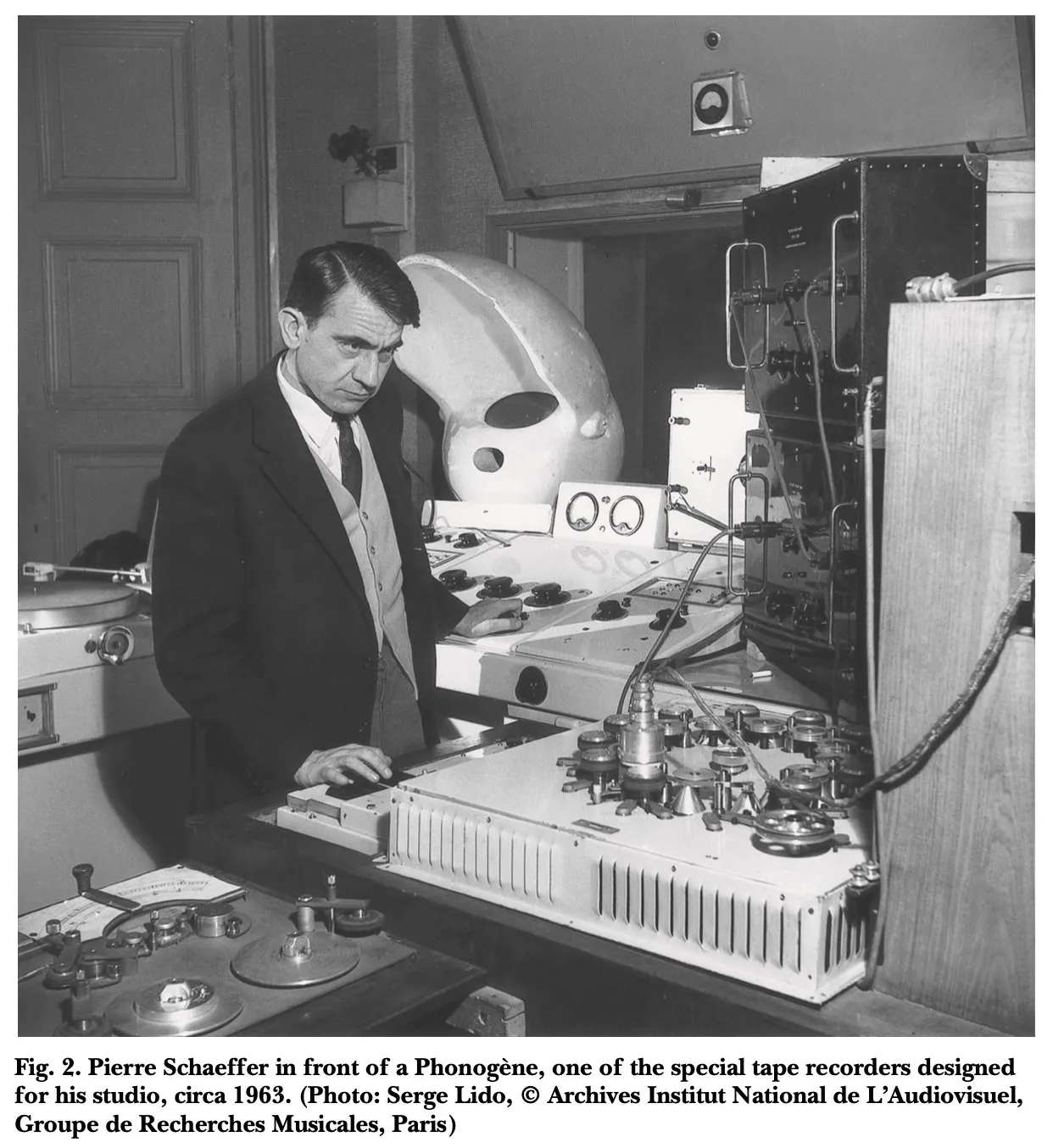
• Musique Concrète was an artistic movement focussed on using recorded sounds.
• Pierre Schaeffer (and team) in France, Post WW2 (1945-1960)
• First using 78RPM records
• Then manipulation of tape
• GRM (Groupe de Recherches Musicales) still exists!

Source: Manning, P. (2003). The Influence of Recording Technologies on the Early Development of Electroacoustic Music. Leonardo Music Journal 13, 5-10. https://www.muse.jhu.edu/article/50703

Why make Musique Concrète?

recordings are a rich sound material

recordings relate to the real world

recordings are flexible and interesting at different scales

getting some sound

Why does sampling work?

What information is there in the sound file?

How do we get some sounds?

Sampling Theory

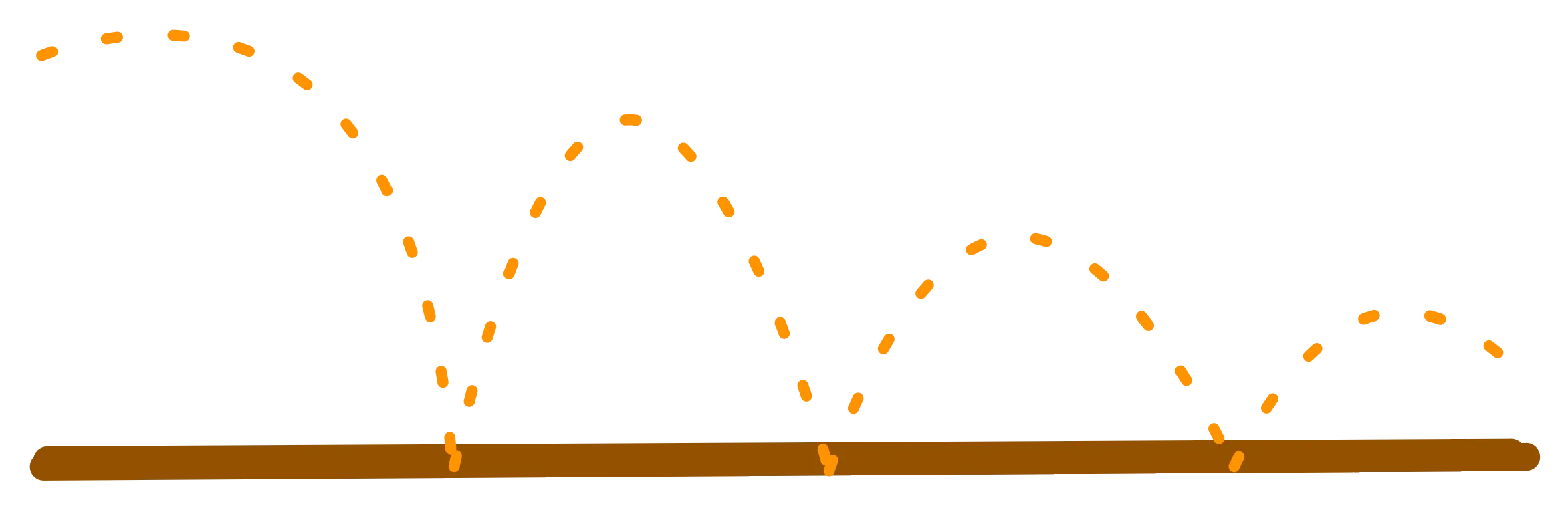
What is the possible path that the ball can take?

There’s only one solution!

As long as the ball doesn’t bounce too fast.

remember the Nyquist-Shannon Theorem:

A signal containing only frequencies lower than B Hz can be (perfectly) reconstructed from samples taken at 2B Hz.

What does it mean for a sound to have frequencies in it?

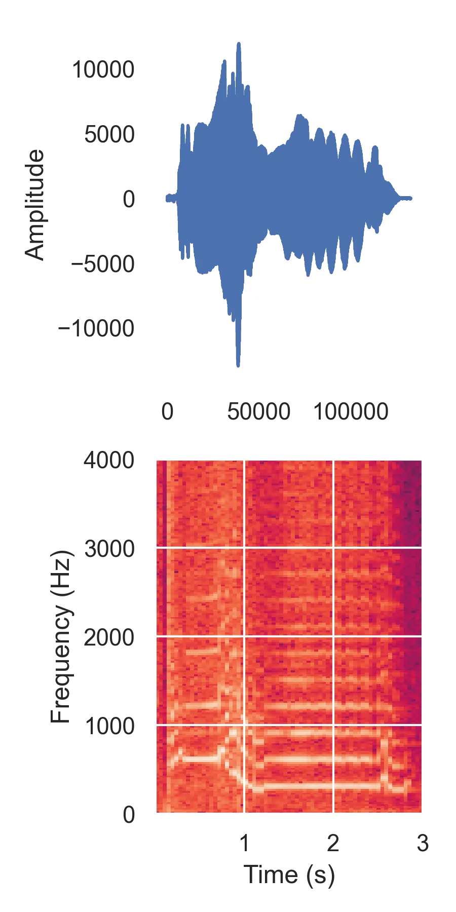
• We can think of complex sounds as combinations of basic sounds.

• The most basic sound is the sine wave (or sinusoid) that we played last week.

• All sound can be represented as a combination of sinusoids with different frequencies, amplitudes (and phases).

• Sounds change over time, which means the amplitudes move up and down.

Defining a sinusoid: the most basic sound

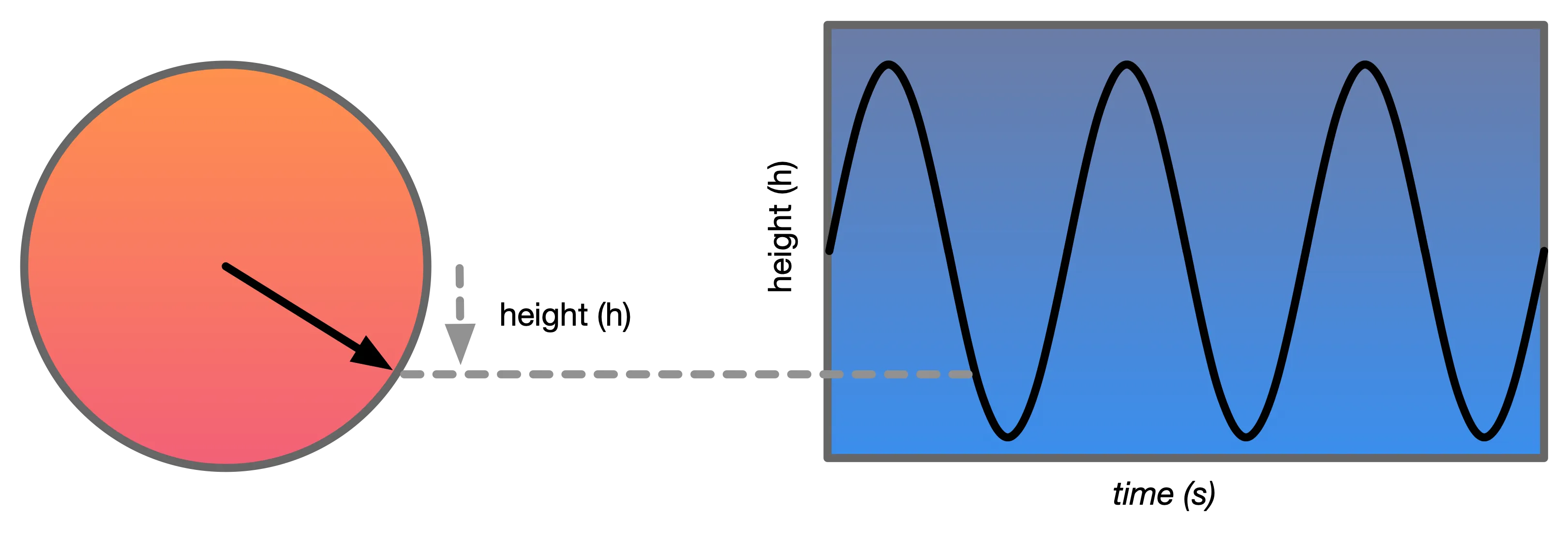
Imagine fixing a point on a spoke of a bicycle wheel as it spins. The height of the moving point from the centre follows a sine wave.

We can write down the height as a function: $h(t) = sin(2 \times \pi \times t)$

Changing the sinusoid

There’s three parameters we can modify in the sinusoid:

• frequency (how fast the wheel spins in cycles per second)
• amplitude (radius of the wheel)
• phase (the point where we started spinning)

We can extend the function: $h(t) = A \times sin(v \times 2\pi t + \phi)$

This formulation is called a phasor.

(a bit of a simplification, but ok for this course! for more, see ENGN4537)

Changing sinusoids

$h(t) = A \times sin(v \times 2\pi t + \phi)$

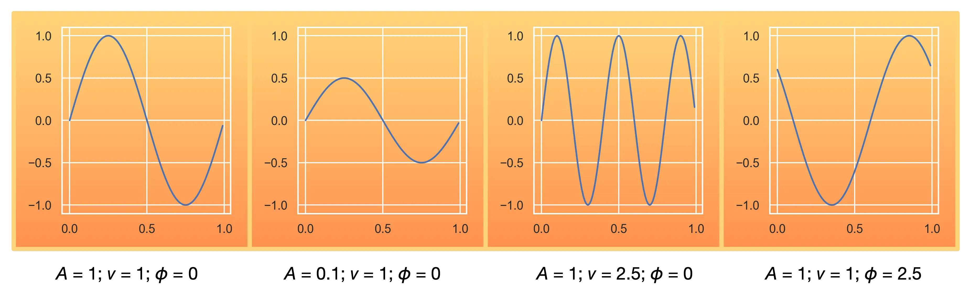
What would the perceptual effect of these changes be on a sound wave?

Fourier Transform

• In around ~1800, Jean Baptiste Fourier figured out that any “periodic” function can be expressed as the sum of a series of sine and cosine terms (i.e., a series of sinusoids).

• A consequence of this is that you can find out the amplitude and phase of the sinusoidal component at a certain frequency.

You can do this with the “Fourier Transform” formulas.

• Warning: maths notation incoming: if you haven’t done 1st year university maths, this will look very confusing.
• The good news is it’s the concept that is important, the maths is presented for completeness

Fourier Transform Formulas

Given a function $f(t)$ and a frequency $\omega$

• The sine amplitude is: $R(\omega) = \int_{-\infty}^{\infty} f(t)cos(\omega t)dt$
• and cosine amplitude is: $X(\omega) = - \int_{-\infty}^{\infty} f(t)sin(\omega t)dt$

The above give us two amplitudes, for out-of-phase sine and cosine waves. These can be rewritten to the amplitude and phase for a sine wave:

• Amplitude: $A(\omega) = \sqrt{R(\omega)^2 + X(\omega)^2}$
• Phase: $\theta(\omega) = arctan(X(\omega) / W(\omega))$

These equations integrate over all t values (time)—so information about time is lost!

Fourier Takeaways

• All sounds can be deconstructed into sinusoids

• Sinusoids have three parameters: amplitude, frequency, and phase

• We can use maths to find the amplitude and phase for a given frequency in an audio signal

• The (big) tradeoff is that information about time is lost.

Everything said above relates to infinitely long continuous signals, not sampled signals. We will come later to details about how to do this with time-limited digital signals.

See Dannenberg Chapter 3 for reference.

Sampling and the Frequency Domain

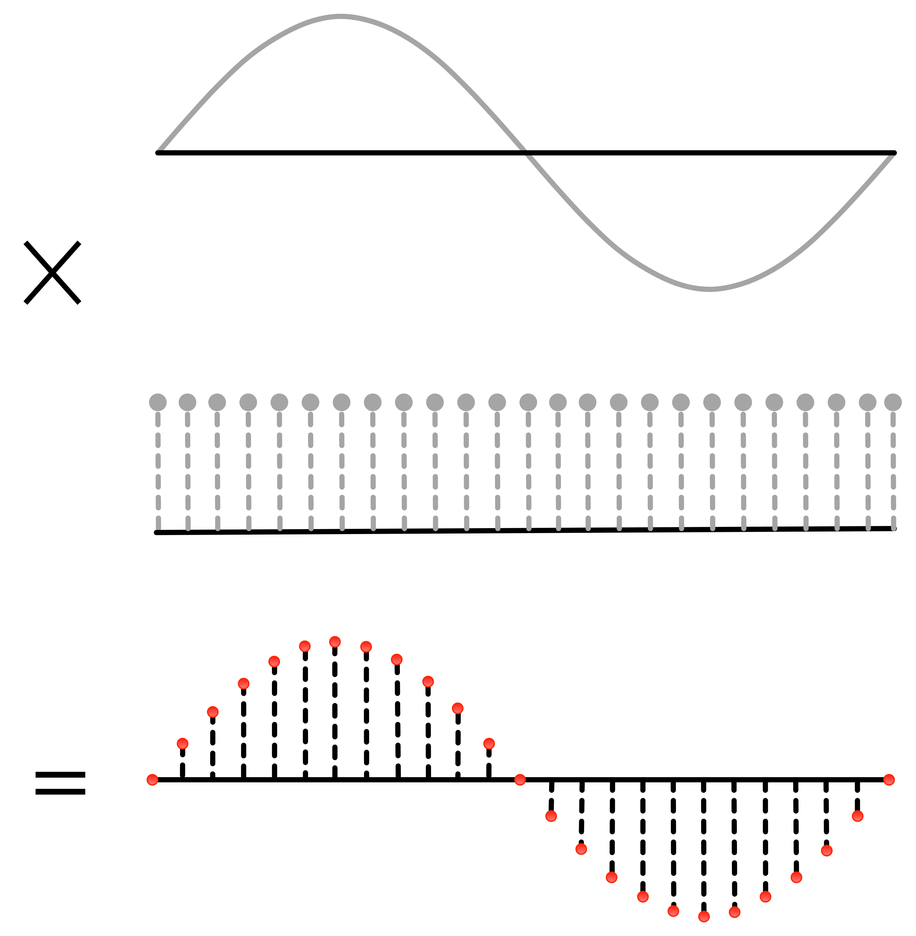
You can look at sampling as a time domain operation.

Create a series of impulses and multiply with the signal to be sampled.

The result is the sampled information.

We hope that in the frequency domain the spectrum of our sound has been preserved.

Spectrum of a sampled signal

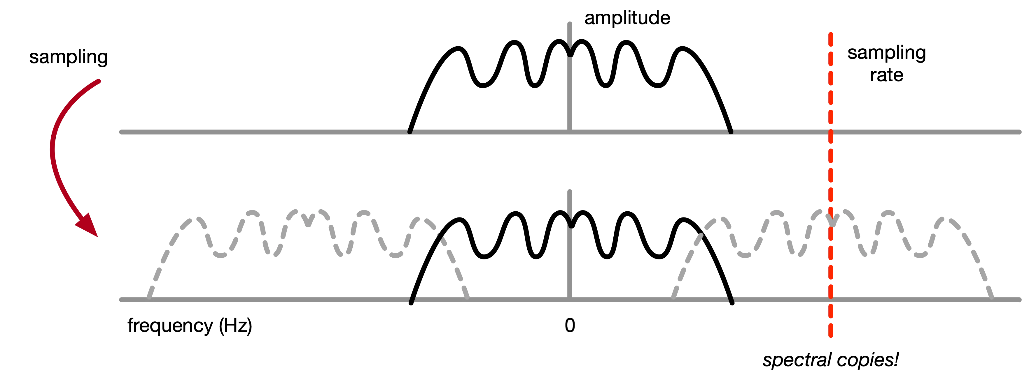
The frequency domain of the sampled signal is really weird.

It turns out the spectrum of the signal copied at each multiple of the sampling rate. This is bad because the copied frequencies interfere with spectrum that we want.

Solution:

• Recorded sound contains all kinds of frequencies that we can and can’t hear.

• Analogue-digital converters filter the sound to make sure that only frequencies below the Nyquist frequency (half the sample rate) are sampled.

• This avoids aliasing in the sampled signal messing up frequencies that we want.

Quantisation Noise

Sampling also involves “rounding” the analogue signal to a digital number.

Digital numbers have a concept of “precision” (how many possible values can be represented).

• An 8-bit number (a byte) can only represent $2^8$ or 256 values
• a 16-bit number can represent $2^{16}$ or 65536 values.

The effect of rounding our samples is to introduce noise into the signal.

• We can measure the difference between the potential amplitude of a signal and the (always present) noise as a signal-to-noise ratio (SNR) in decibels (dB).
• Roughly 6dB per bit.

CD Quality Audio:

Now you know why digital audio is often recorded at 44.1kHz sample rate and 16bit sample depth:

• 44.1kHz: more than double 20kHz which is the maximum frequency humans can perceive to avoid audible aliasing.

• 16-bit sample depth: gives ~98dB SNR so that we can’t hear noise in a well-prepared signal.

These values are often called “CD quality” audio as they were specified for the CD digital format (in 1982). They give extremely high-quality audio.

let's go do it

time to make some Musique Concrète with soundfiles in Pd

we need a sound in WAV format…

let’s find one: https://freesound.org/browse/random/

other options: record a sound on your phone

Simply playing back sound files

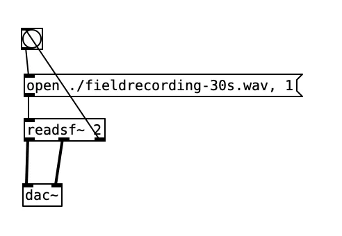
You can use readsf~ to open and play back a sound file. Is that enough??

• readsf~ is easy and convenient, but limited

• reads from your hard drive

• can’t change speed or playback position (crucial for Musique Concrète)

More sophistication and fun: reading a sound file array

Best way to make music with sound files:

1. load the data into an array variable using the soundfiler object
   • Make a graphical array from the “Put” menu
   • Make an array with no GUI with the array object: [array define {array-name}]
2. use the tabread4~ (table read) to play audio data from any point in the array

tabread4~ is like the read head of a tape machine: it just accesses the data, it doesn’t move the tape

need to use other objects (e.g., phasor~ or line~) to “move” tabread4~ up and down the tape.

Musique Conrète with tabread4~

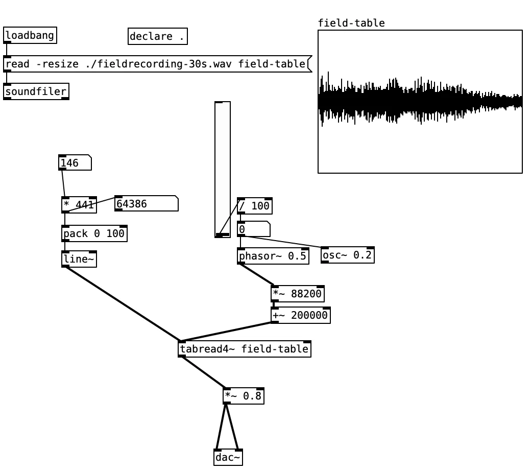
1. load file into an array with soundfiler
2. set up a tabread4~ object to access the table
3. use a phasor~, or any other audio rate object to playback bits of the file.
4. you can even just scribble around in the file with line~

Wavetable-lookup synthesis

making an oscillator from a soundfile

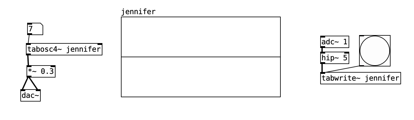
• tabosc4~ scrolls through a (whole) array at a certain frequency.
• this is a basic way of doing wavetable synthesis which includes the idea of evolving the array over time (in some way)
• read up on classic wavetable synthesis if you want.

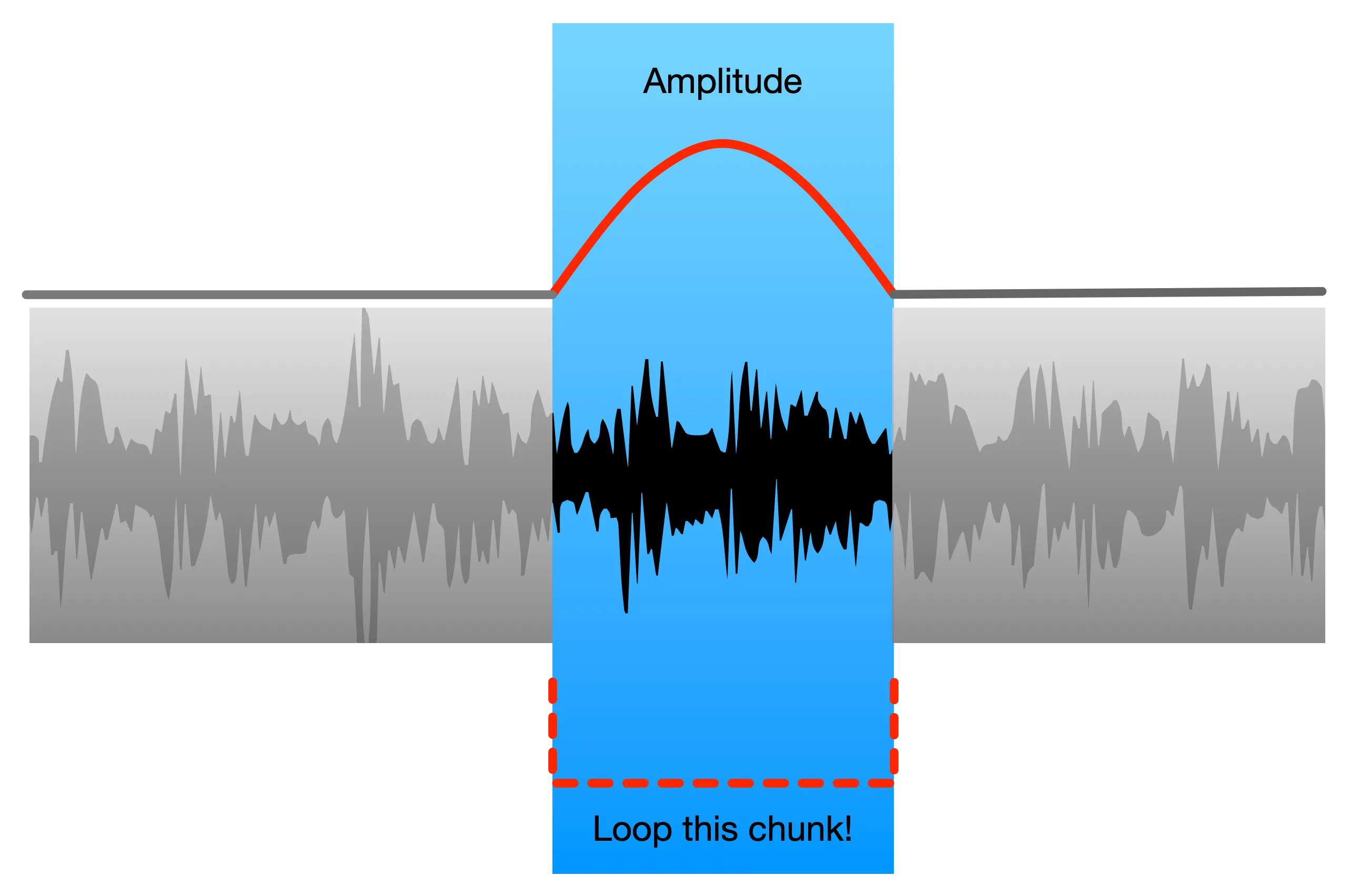
Looping Grains of Audio

Granular Synthesis in Pd

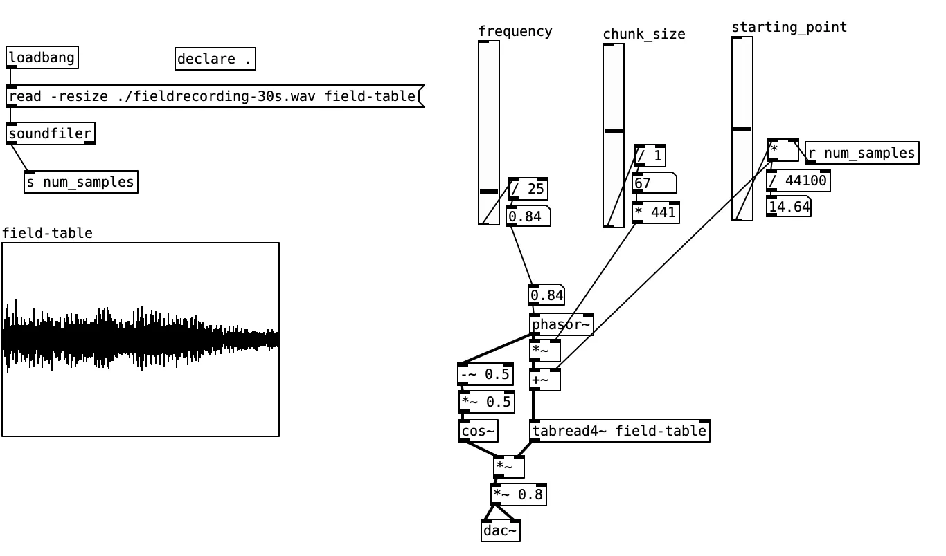
• Loop a bit of a soundfile over and over to make a continuous sound.
• Note the cos~ bit here to avoid clicks at the start and end of the looped section.
• See B13.sampler.overlap in the Pd help for a better version.
• See Dannenberg Chapter 6.2 for more.

Sampling in Strudel

How can we play back sounds in Strudel?

// Load a sample (shortcut method for GitHub)
samples({'field':'1-digital-synthesis/fieldrecording-30s.wav'},
        'github:cpmpercussion/ComputerMusicIntro')
// Play back from different starting points
s("field").begin("<0 .25 .5 .75>").clip(1)

This shows just one way to load a custom sound (from GitHub) and one way to play back different sections.

Granular Synthesis in Strudel

It’s not easy to replicate the Pd example exactly in Strudel, but we can do other cool stuff…

samples({'field':'1-digital-synthesis/fieldrecording-30s.wav'},
        'github:cpmpercussion/ComputerMusicIntro')

note("60").slow(2)
  .add(note("0,.63")) 
  .s("field").begin(rand.range(0,0.9)).clip(1).speed(rand2)
  .lpq(8).lpf(400).lpa(.2).lpenv(4)
  .room(.5)

This plays notes starting at random points in field at random speeds with a filter envelope, reverb, and detuning to enhance the timbre.

Checklist for the day:

Have you:

• played back your own soundfile in Pd?
• tried out tabread4~ in Pd and understood how to control it with line~ and phasor~?
• tried out the granular synthesis patch in Pd?

Links and References for the day:

• Dannenberg Chapter 3 “Sampling Theory Introduction”
• Dannenberg Chapter 6.2 “Granular Synthesis”
• Kreidler Chapter 3.4 “Sampling” (Pd examples)
• Kreidler Chapter 3.6 “Granular Synthesis” (Pd examples)
• Sound on Sound Apr. 98. Synth School, Part 7: Transitional Synthesis
• Seeing Circles, Sines, and Signals - a primer on DSP (if you want to start knowing more about FT and sampled audio)