Outline

• Filters (analogue, digital, vcf~, bob~, filter math (light)
• Subtractive Synthesis (from phasor to Moog Model-D clone))
• FM Synthesis (recall week 3, feedback, algorithms, operator-based design)
• Phase Vocoder + spectral synthesis.

Subtractive Synthesis

Subtractive Synthesis

Let’s take a complex sound and remove some content.

Popular Subtractive Synths

Subtractive synthesis is often used in analogue synth designs, particular with those associated with Bob Moog (famous synth designer).

E.g.,:

• Minimoog Model-D (1970)
• Moog Mother 32 (2015) ~AUD1100
• Korg Volca Keys (2013) ~AUD250
• Arturia Microfreak (2014) ~AUD550

It’s good for analogue designs because you can get a lot of timbral variation out of few (2 or 3) basic oscillators.

Subtractive Synth Layout

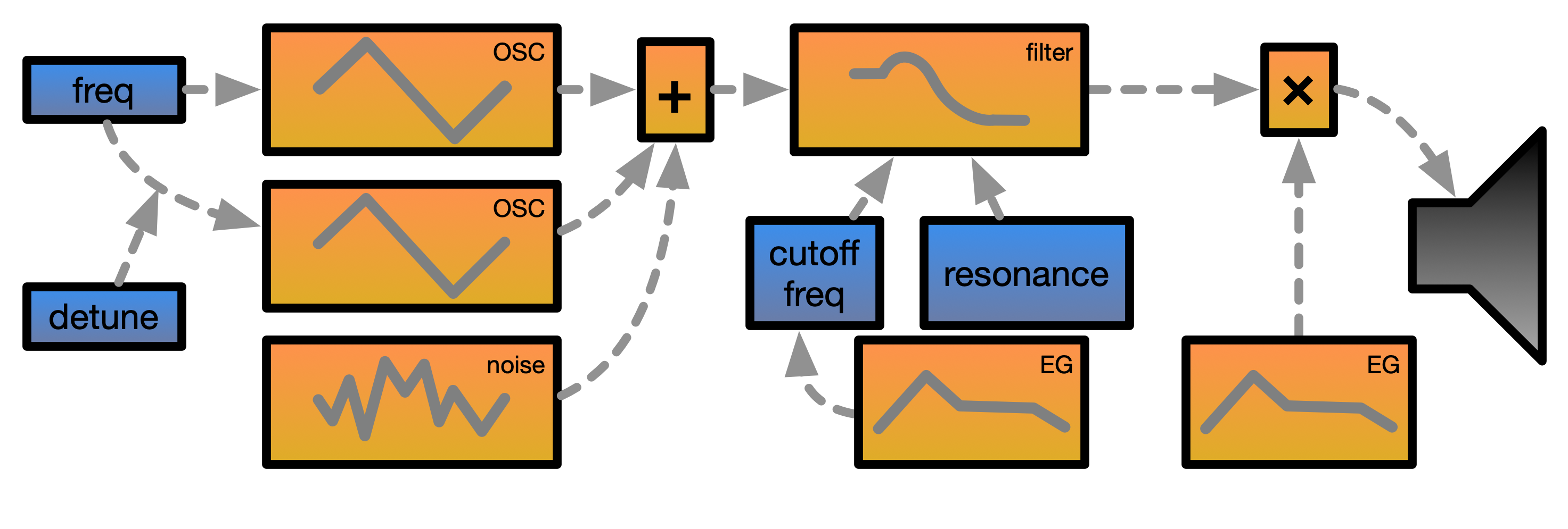
• Sound is produced by 1+ summed oscillators and/or noise generator, processed by filter
• Two envelope generators: output volume and to change the filter cut-off frequency
• Missing: low frequency oscillator for modulation

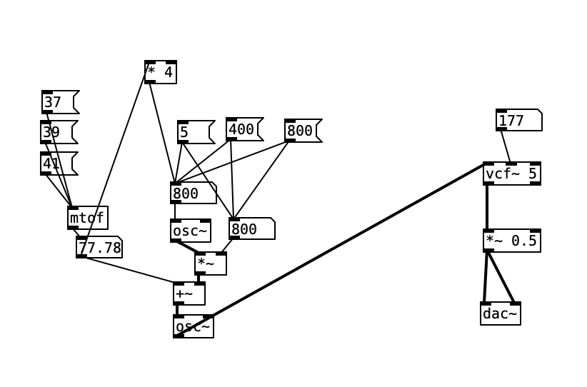
Minimoog in Pd

Here’s a basic design for an analogue synthesiser with two sawtooth oscillators.

• “detune” changes the frequency of the second oscillator, try a number close to 1, e.g., 1.05 for a rich phase-y sound.
• the filter env gives the sound a nice changing timbre over a note
• for extra fun, try the bob~ object. Similar to vcf~ but modelled on actual Moog filter designs.

N.B.: the synthesis part here is quite simple, but processing note information is tricky and requires lots of supporting objects.

FM Synthesis

Simple two-oscillator FM

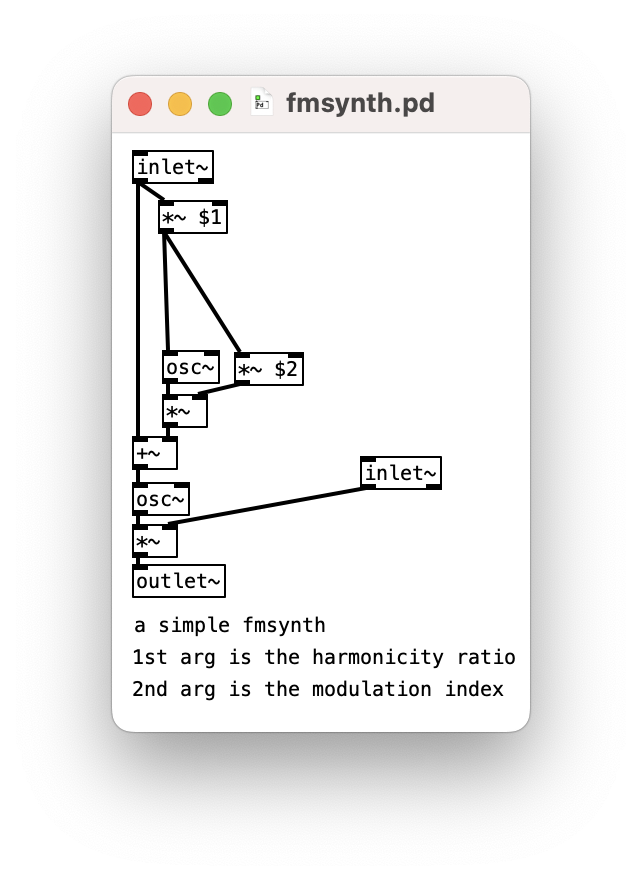
We introduced FM synthesis earlier in the course as a way to make interesting sounds with just two oscillators.

This fmsynth.pd patch has been used a lot!

• $1 is harmonicity (modulation frequency divided by carrier frequency)
• $2 is the index (modulation depth divided by modulation frequency)

This allows us to create a consistent timbre for any frequency input. Can we do more with more oscillators?

Revision: Phase Modulation

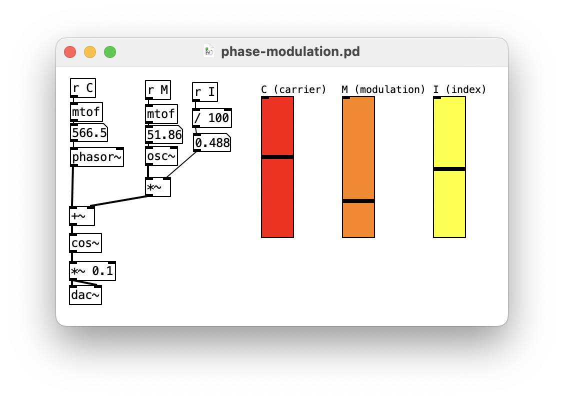
Let’s just revise how “frequency modulation” works.

• FM can be implemented by modifying the phase of an oscillator.
• In this patch, the phase is modified in between the phasor~ and cos~ objects.

FM Operators

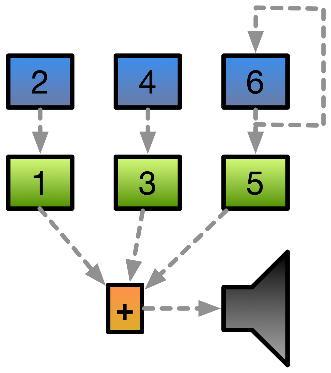
We can take the concept of a phase-modulation oscillator and abstract to a reuseable unit: an FM operator.

• An op can serve as a carrier, or as a modulator.
• An op can self-modulate (crazy sounds).

Combining multiple oscillators allows lots of sounds to work together. Typical FM synths will have 4 or 6 operators.

In FM lingo, the wiring diagram between operators is called an algorithm.

Implementing 6-op FM

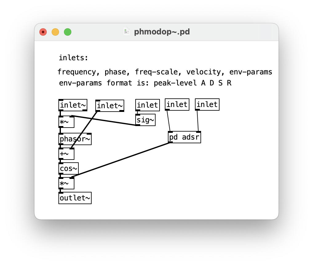
Each operator needs:

• an envelope generator
• amplitude and envelope parameters
• some pitch-ratio control
• pitch ratio parameters

This gets complicated quickly…

Volca FM has 23 parameters per operator, and 16 global parameters, that’s 154 params for one patch!

Operator Layout

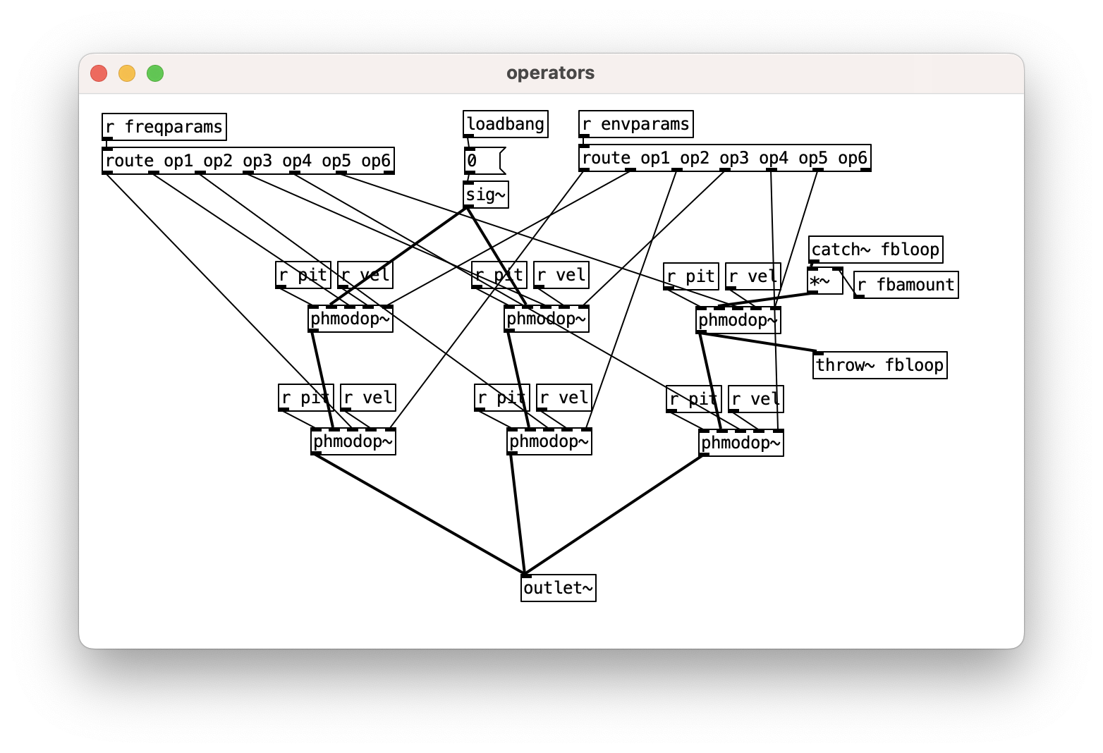
And here’s how you could wire them together…

• note that every op gets the pitch and velocity signals
• using r and route to send freq scaling and envelope parameters
• throw~ and catch~ for the feedback loop on operator 6.

This is a fixed configuration, could you design a way to control the FM algorithm with parameters?

Commercial FM Synths

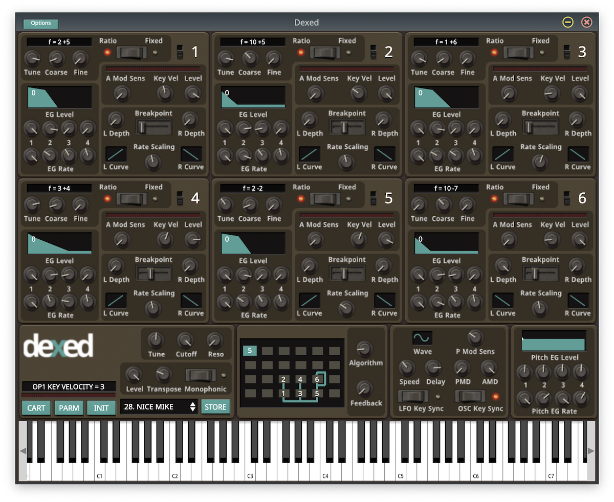
Op-based FM is very popular. The Yamaha DX7 was the first successful digital synthesiser in 1983 and Yamaha’s FM sound chips were found in computers and video game consoles throughout the late 80s and 90s.

• Yamaha DX7 (1983)
• Yamaha reface DX (2015) ~AUD600
• Korg Volca FM (2016) ~AUD250
• Elektron Digitone (2017) ~AUD1350
• dexed FM Plugin (modeled on DX7) AUD0

See dexed for free FM synth fun.

String Synthesis

Karplus-Strong string synthesis is a famous algorithm for creating a string-like sound with a noise source, a delay and a filter.

It can be considered a special case of digital waveguide synthesis, used for string, tube, and membrane sounds.

K-S synthesis is quite common in digital synthesisers (e.g., Arturia Microfreak) and it’s fun to do in Pd.

Pd String Synthesis

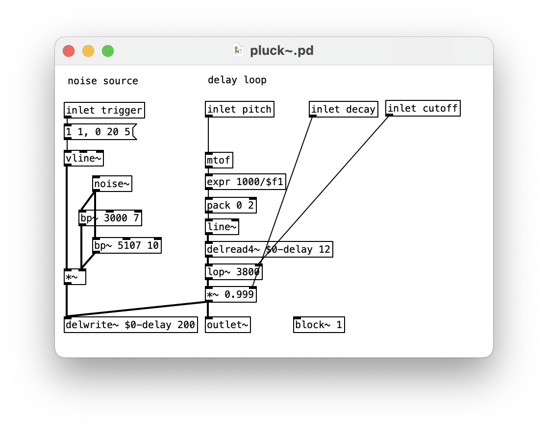
Here’s a simple Karplus-Strong implementation.

• Noise source is some lightly filtered noise~
• vline~ controls noise entering the delay loop
• the delread~ and delwrite~ define the delay loop
• the filter is a lop~, and the loop has feedback of 0.999
• changing the length of the delay loop changes the pitch, so this is adjusted by the frequency input

Physical Modelling Synthesis

Physical modelling synthesis is an interesting area with lots of possibilities and challenges.

Have a look at Julius O Smith’s Stanford Courses (Music 420A) to learn more.

Fourier Resynthesis

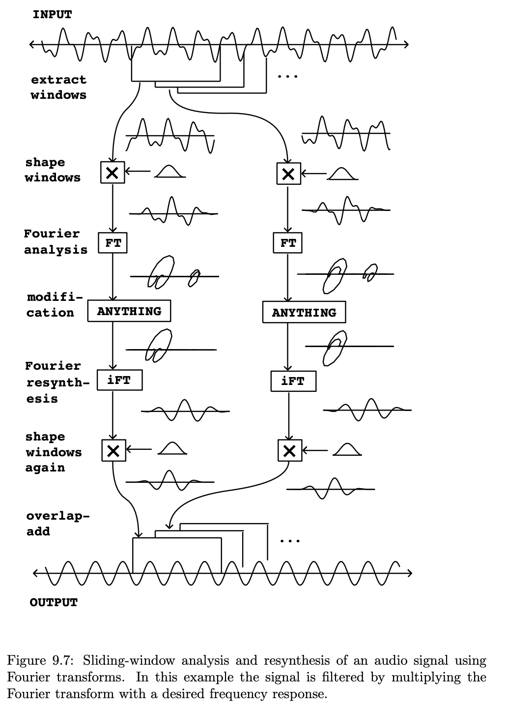
One form of synthesis that is usually limited to computers involves modifying the frequency domain of a sound and recreating new versions.

Spectral manipulation is something that Pd is quite good at doing!

We return a bit to the Fourier transform mentioned early in the course.

For the full story, see Fourier Analysis and Resynthesis in Miller Puckette’s book.

Back to the frequency domain

Remember the Fourier transform? This allowed us to extract the amplitude each frequency component of a sound.

In practice, the FT can’t be used as it requires an infinite input (who has time for that).

We can use a similar construction called: Short-Time Discrete Fourier Transform (STDFT):

• short-time: operates on a finite-length signal instead of an infinite signal

• discrete: operates on sampled information

We often refer to SDTFT as FFT, or “fast Fourier transform” (e.g., the fft~ object in Pd). FFT is actually a clever algorithm for accomplishing a DSTFT quickly, so it’s ok to use the acronyms interchangeably.

Short-Time Discrete Fourier Transform

For a signal with $N$ samples, the STDFT equations providing the sine and cosine amplitudes at certain frequencies are:

• $R_k = \sum\limits_{i=0}^{N-1} x_i cos(2\pi k i \ N)$

• $X_k = - \sum\limits_{i=0}^{N-1} x_i sin(2\pi k i \ N)$

The STDFT also only focuses on $N$ frequencies that we call “bins” between 0 and the sampling frequency.

• If the sampling rate is $S$ then the frequency of the $k$th bin is: $k * \frac{S}{N}$

N.B.: the frequency “resolution” is limited by the length of the signal we are analysing!

FFT on a long signal

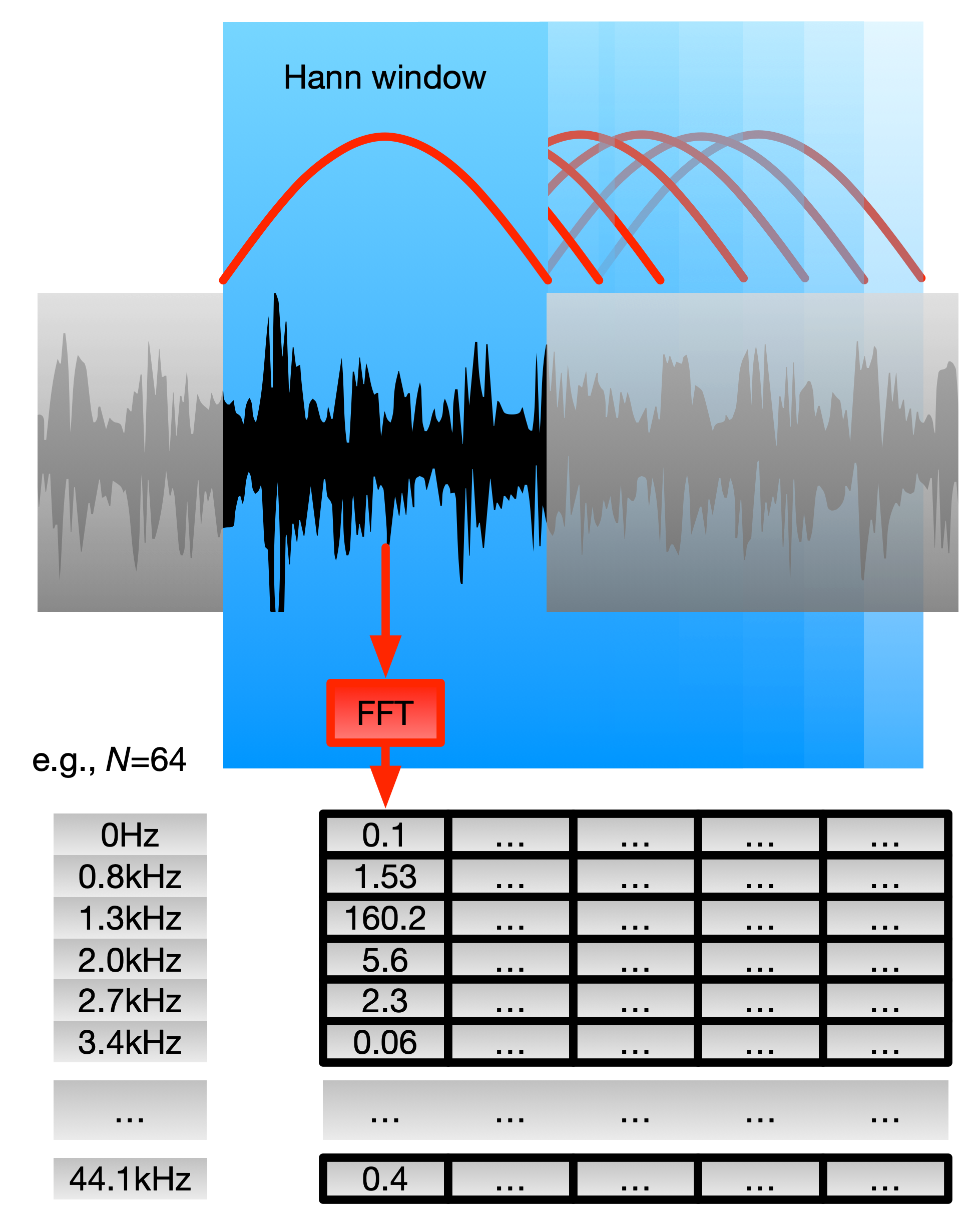
Typically we want to apply FFT to a “chunk” of a signal rather than the whole thing.

Usually we can set the length of the chunk (window length) and an envelope function.

The usual choice for envelope function is the Hann function, it looks kind of like a Gaussian distribution.

The window length is flexible, but will determine the number of frequency bins that can be analysed! Usually the window length is required to be a power of 2 (e.g., 512 or 2048)

Inverse FFT

The FFT procedure actually also works backwards!

• From a finite sequence of frequencies we can (re-)create a sampled signal!

The exclamation mark is doing a lot of work here! Imagine what we can do with full control over a spectrum!!

In fact, the IFFT algorithm is almost identical to the FFT algorithm

It is important when doing an FFT to cope with the sine and cosine elements (or the real and complex outputs of a frequency. These interact in a certain way to make the ouput sound “work”.)

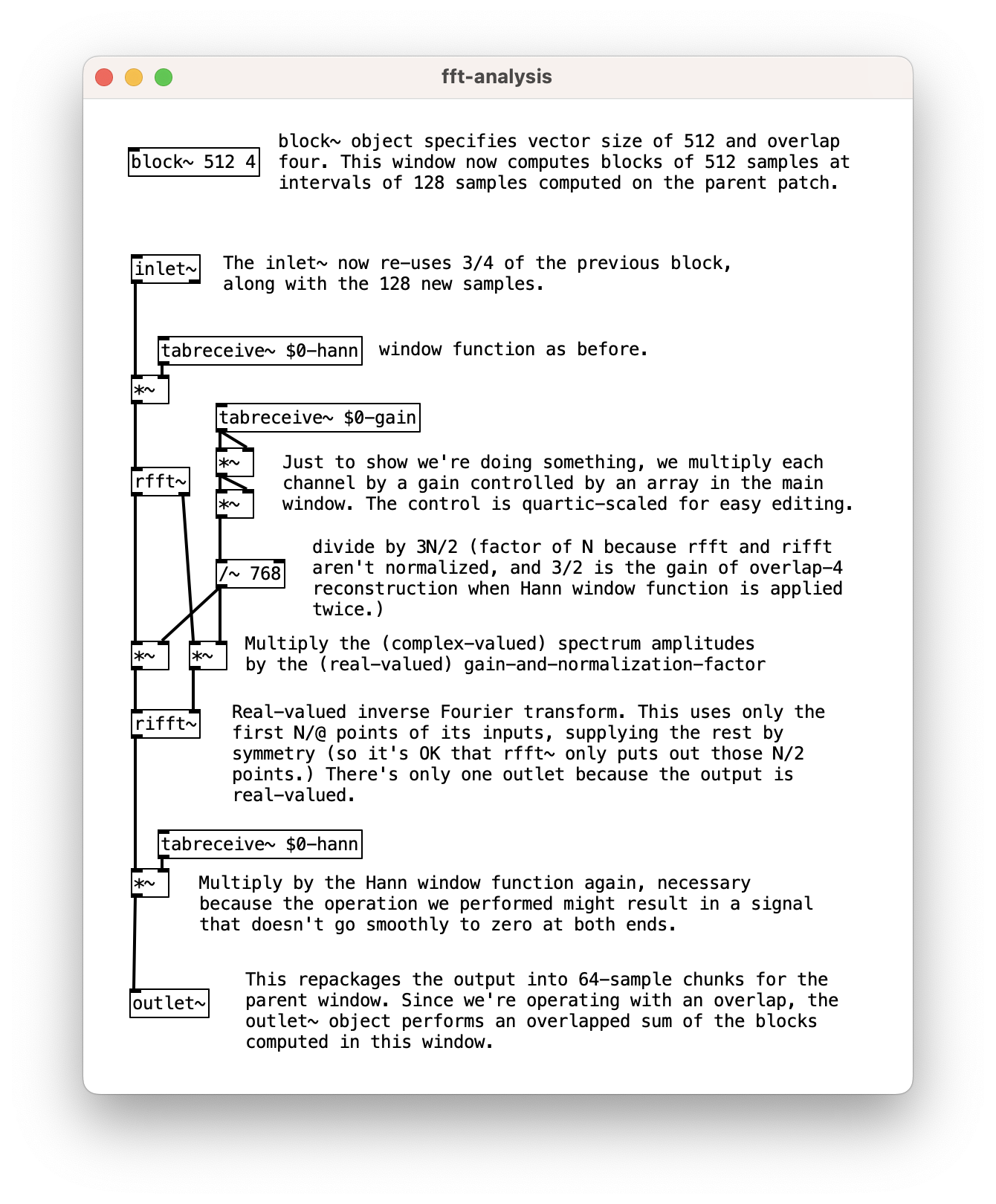
FFT in Pd

Pure Data can perform a STDFT with the fft~ object (yes it’s that easy).

The two outputs give you the real and imaginary part of the signal. You can also do rfft~ just to get the real output (saves CPU).

Similarly, you can do an inverse FFT with rifft~ and ifft~.

In Pd, N is the same as the “block size” (number of samples processed at once), so Pd patches often adjust block size just for the FFT patch to get the right number of FFT bins.

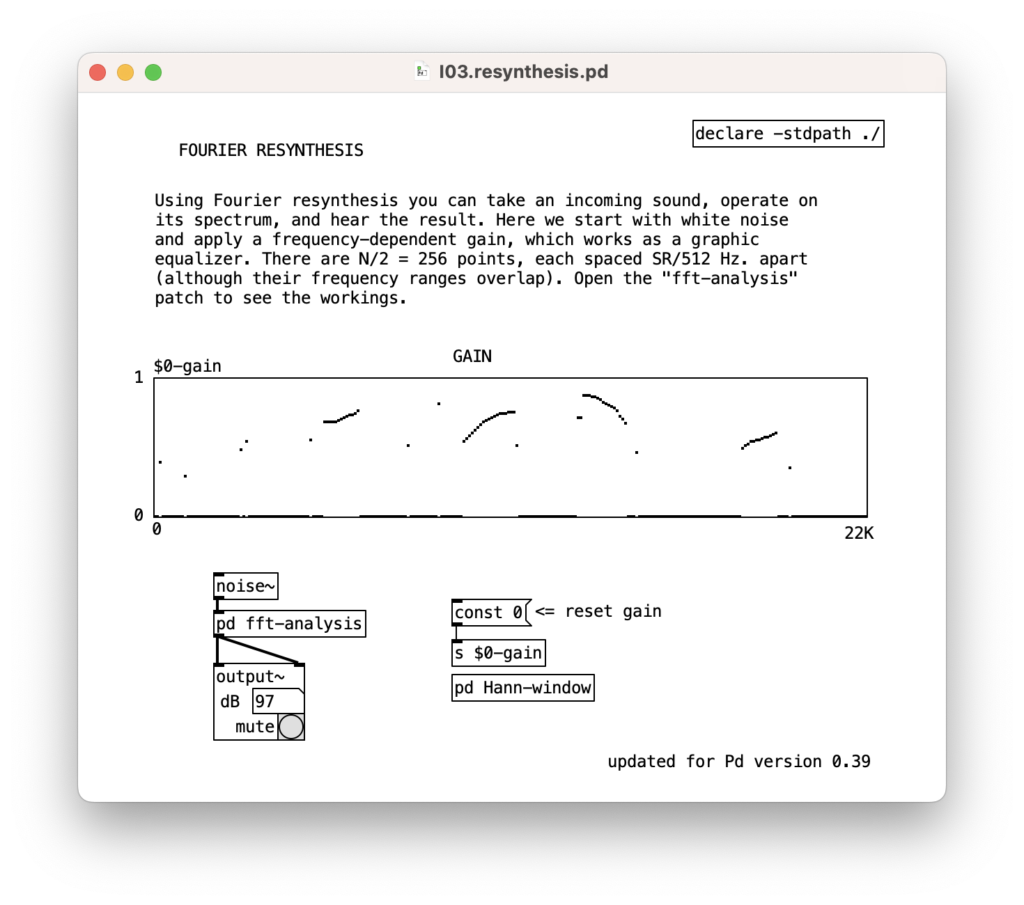
Basic Resynthesis

Here’s a fun way to modify the spectrum of “noise”.

Timbre Stamp

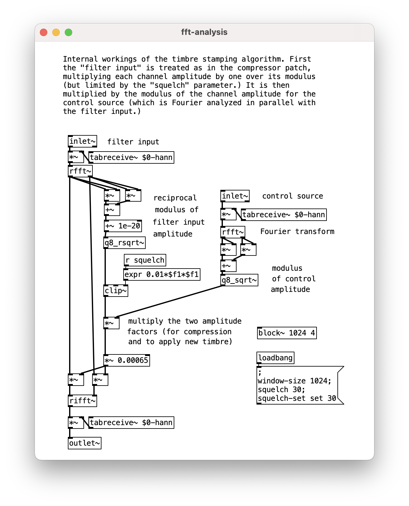
The “timbre stamp” algorithm modulates a signal by the spectral envelope of another sound.

see I06.timbre.stamp.pd

Phase Vocoder

The “phase vocoder” is an algorithm for stretching or compressing the time and frequency axes of a recorded sound.

see I07.phase.vocoder.pd