COMP1730/6730 Project Assignment

Last update: 25/09/2023

In this assignment you will develop a program to simulate the motion of a planetary system, such as our Solar system, in which we will project the movements in three-dimensional space onto a 2-dimensional plane.

Practical information#

The project assignment is due Sunday, 15th October 2023 at 11:55pm (end of week 10). To submit your solution, you have to upload via wattle:

A single Python source file.
A report with your answers to a set of predefined questions. Details about the format of the report and the questions are provided in the section Questions for the individual report below.

Here is the assignment submission link.

NOTE: You must attend the lab in week 11 to discuss your solution with a tutor. If absent without prior approval by the convener, you will receive zero mark.

NOTE: No excuses about technical problems like Internet connection or computer issues are accepted. You can actually submit the assignment as many times as you like, as the last submitted file will be marked. Do not wait until the last minute!

The project assignment is individual. You must write your own solution, and you are expected to be able to explain every aspect of it. You are not allowed to share your solution (code) with other students; this includes posting it (or parts of it) to the discussion forum, or to any other on-line forum.

If you have questions:

Ask the tutor in your lab,
Look at the Wattle discussion forum for a similar question, and only post your question if not found,
Go to drop-in sessions.

Background#

While the planets are obviously moving in a 3-dimensional space, it turns out that all eight planets in the Solar system nearly orbit in the same 2-dimensional plane (the ecliptic plane relative to the Sun). This observation allows us to simulate their trajectories in the 2D space. More generally, we want to model the movement of any planetary system in 2D, not just our Solar system. Each star/planet can be represented as a point in this 2D plane with coordinates (x,y).

Storing configuration of a planetary system#

Before doing any motion calculation we need to know the current configuration of the star and the planets, including their masses, positions and velocities in the planetary system. The file solar_system.tsv provides a real example of the configuration of our Solar system on 1st May 2020:

Name	Mass	XPOS	YPOS	XVEL	YVEL
Sun	1.99e+30	0.00e+00	0.00e+00	0.00e+00	0.00e+00
Mercury	3.30e+23	4.51e+10	1.99e+10	-2.80e+04	4.72e+04
Venus	4.87e+24	-1.02e+11	-3.47e+10	1.14e+04	-3.32e+04
Earth	5.97e+24	-1.15e+11	-9.75e+10	1.90e+04	-2.27e+04
Mars	6.42e+23	2.87e+10	-2.12e+11	2.49e+04	5.39e+03
Jupiter	1.90e+27	2.10e+11	-7.45e+11	1.24e+04	4.18e+03
Saturn	5.68e+26	6.54e+11	-1.35e+12	8.15e+03	4.19e+03
Uranus	8.68e+25	2.38e+12	1.76e+12	-4.09e+03	5.16e+03
Neptune	1.02e+26	4.39e+12	-8.95e+11	1.05e+03	5.36e+03

This file is in tab-separated format with six columns. The first line is the header line showing the name of the columns and each of the remaining lines corresponds to a star/planet. The column meanings are:

Name: Name of the star/planet.
Mass: Its mass (kilograms).
XPOS: x-coordinate (in meters) of the star/planet.
YPOS: y-coordinate (in meters) of the star/planet.
XVEL: x-velocity (in meters/second), the speed at which the star/planet is moving on the x-axis.
YVEL: y-velocity (in meters/second), the speed at which the star/planet is moving on the y-axis.

We use the standard SI units for all quantities, i.e., time, mass, velocity, acceleration, etc.

You can use the plot_configuration function provided in the skeleton file to visualise the configuration. For the solar_system.tsv you should see the following figure:

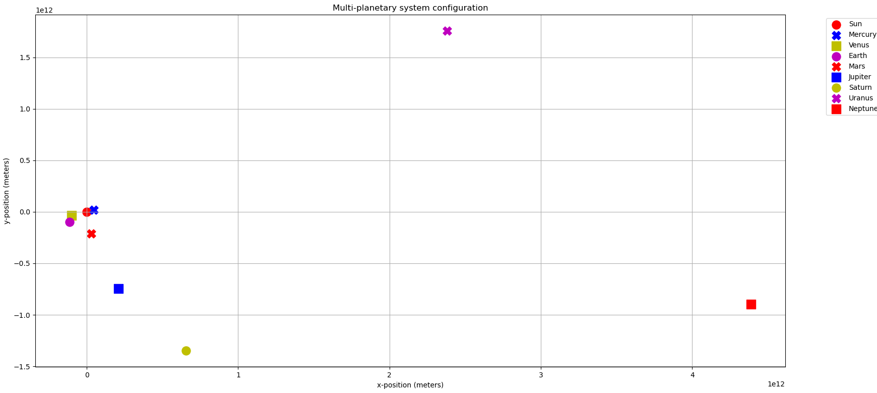
NOTE: You cannot assume that there are always 1 star and 8 planets with these names in a configuration file. In fact, we will test your code with other planetary systems such as trappist-1.tsv, which corresponds to the so-called TRAPPIST-1 multi-planetary system (discovered during the 21st century). However, you can assume that the header line will stay the same for all testing files.

Questions for analysis (code)#

A template file for the assignment code is provided here:

assignment.py

In this file, there are several functions that you must implement for tasks 1-4 for COMP1730 students and tasks 1-5 for COMP6730 students. These functions only have a pass statement that you should replace with your own implementation. You do not have to solve all the tasks, but you can only gain marks for the ones that you have attempted (see Marking criteria below for details on how we will mark your submission).

Task 1: Predicting the configuration after a certain time#

The configuration of the planetary system that you read from the file provides the initial positions of the star/planets at the relative time point \(t_0 = 0\). That means, from now on we measure time as relative to the time of measurement of the initial configuration. We now want to predict the configuration at a “future” time point \(t_1\) (in seconds).

Let’s assume there are \(k\) star/planets that are indexed from \(0\) to \(k-1\). In the Solar system example above, \(k\) is 9. From now on we will just call a star/planet as an astronomical object, or object for short. Let \(\mathbf{p}_i = (x_i, y_i)\) be the position of the object \(i\) at the current time point \(t_0\). You can store \(\mathbf{p}_i\) as a sequence of two numbers, which can be a list, a tuple, or a NumPy array of two numbers (or any other datatype that you like).

Let \(\mathbf{v}_i\) be the velocity of the object \(i\) at the current time point \(t_0\). Because objects are moving in 2D space, \(\mathbf{v}_i\) is represented as a sequence of two numbers, like \(\mathbf{p}_i\). The sequence type is of your choice, but we recommend to use the same type as \(\mathbf{p}_i\).

From high school physics, if all objects are moving at a constant velocity during the time period from \(t_0\) to \(t_1\), then the new position of object \(i\) at \(t_1\) should be:

\[\mathbf{p}^{NEW}_i = \mathbf{p}_i + \mathbf{v}_i \cdot (t_1 - t_0).\]

Example: For the example Solar system above, the Earth’s position is (-1.15e+11, -9.75e+10) and it is moving at velocity (1.90e+04, -2.27e+04). Its new x- and y-coordinate after 1 day (86400 seconds) are:

x = -1.15e+11 + 1.90e+04 * 86400 = -1.133584e+11 y = -9.75e+10 + -2.27e+04 * 86400 = -9.946128e+10.

Task 1: Write a function compute_position in the template Python file that takes two parameters: (1) a string for the path to a file storing the configuration of a planetary system and (2) a floating-point number for the time (in seconds). It should return a table with \(k\) rows and 2 columns, each row \(i\) stores the position of object \(i\) at the new time point. The order of the rows should follow the order of objects in the input file. The returned table can be a list of lists, a 2D NumPy array, or any other type, provided that we can access its elements using table[i][j] syntax.

Testing: You can use the test_compute_position provided in the template Python file to test your implementation. Note that it is only testing a limited number of cases and thus does not guarantee the correctness of your code.

Task 2: Computing accelerations#

Task 1 is based on the assumption that the objects are moving at a constant speed. However, this is not true, especially for a long period of time. In fact, all objects are moving at varying velocity. This variation of velocity is caused by the acceleration resulting from the gravitational forces between the objects.

We now want to compute \(\mathbf{a}_i\), the acceleration of the object \(i\) at the time point \(t_1\). Like the positions and velocities, \(\mathbf{a}_i\) is a sequence of two numbers for the accelerations along the x-axis and y-axis of our 2D coordinate space, respectively. To do so, we need to compute the total force \(\mathbf{F}_i\) on object \(i\) by all other objects (except itself) at that time point. Again, the force is represented by a sequence of two numbers for the force on x-axis and y-axis.

For any two objects \(i\) and \(j\), the gravitational force \(\mathbf{f}_{ij}\) between them depends on their masses (higher mass causes larger force) and the distance \(d_{ij}\) between them (smaller distance causes larger force). Here, the (Euclidean) distance between two objects \((x_i,y_i)\) and \((x_j,y_j)\) is:

\[\sqrt{(x_i-x_j)^2 + (y_i-y_j)^2}.\]

\(\mathbf{f}_{ij}\), with \(i \neq j\), is computed as:

\[\mathbf{f}_{ij} = \frac{G m_i m_j}{d_{ij}^2} \cdot \frac{\mathbf{p}_j-\mathbf{p}_i}{d_{ij}},\]

where \(G\) is the gravitational constant \(6.67\cdot 10^{-11}\) (in \(m^3 kg^{-1} s^{-2}\)); \(m_i\) and \(m_j\) are the mass of object \(i\) and \(j\), respectively.

Now the total force \(\mathbf{F}_i\) on object \(i\) will simply be the sum of \(\mathbf{f}_{ij}\) over all other objects \(j\) in the planetary system. The acceleration \(\mathbf{a}_{i}\) of object \(i\) is then given by:

\[\mathbf{a}_{i} = \frac{\mathbf{F}_{i}}{m_i},\]

according to the Newton’s second law of motion.

Task 2: Write a function compute_acceleration in the template Python file that takes two parameters: (1) a string for the path to a file storing the configuration of a planetary system and (2) a floating-point number for the time (in seconds). It should return a table with \(k\) rows and 2 columns, each row \(i\) stores the acceleration of object \(i\) at the new time point. The order of the rows should follow the order of objects in the input file. The returned table can be a list of lists, a 2D NumPy array, or any other type, provided that we can access its elements using table[i][j] syntax. This table is in a similar format to that returned by the compute_position function.

Testing: You can use the test_compute_acceleration provided in the template Python file to test your implementation. Note that it is only testing a limited number of cases and thus does not guarantee the correctness of your code.

Task 3: Forward simulation#

In a forward simulation, we are given a configuration of the planetary system at a time point \(t_0 = 0\), and we want to predict the positions of all objects at a series of “future” time points \(t_1\), \(t_2\), etc.

To do so, you can first predict the object positions at \(t_1\) using your implementation for task 1, then compute their accelerations at \(t_1\) using your implementation for task 2, then compute the velocity at \(t_1\) by:

\[\mathbf{v}^{NEW}_i = \mathbf{v}_i + \mathbf{a}_{i} \cdot (t_1 - t_0)\]

If we now continue to the second time point \(t_2\), we will need to compute the configuration at \(t_2\) based on the configuration from \(t_1\) and NOT from \(t_0\): The above equations for \(\mathbf{p}^{NEW}_i\) and \(\mathbf{v}^{NEW}_i\) are more accurate with lower difference between the two time points \(t_1 - t_0\) as opposed to \(t_2 - t_0\). That means, you can compute the positions at \(t_2\), use these to compute the accelerations at \(t_2\), and compute the velocities at \(t_2\). This can be repeated for next future time points \(t_3\), \(t_4\), etc.

Task 3: Write a function forward_simulation that takes three parameters: (1) a string as the path to a file storing the configuration of a planetary system, (2) a float as time interval \(T\) in seconds, and (3) an integer \(n\). Here the input configuration file corresponds to the time point \(0\). The function should return a table with \(n\) rows and \(2 k\) columns, where row 0 stores the configuration of the planetary system at time point \(\frac{T}{n}\), row 1 for time point \(\frac{2 T}{n}\),…, and the last row for the time point \(T\). The 1st and 2nd columns store the x and y-coordinates of the first object, the 3rd and 4th columns, the coordinates of the 2nd object, and so on and so forth. The order of the objects in the table should follow the input configuration file. You can store the table as any data type such as a list of lists, a 2D NumPy array, or any other type, provided that we can access its elements using table[i][j] syntax.

Testing: You can use the test_forward_simulation provided in the template Python file to test your implementation. Note that it is only testing a limited number of cases and thus does not guarantee the correctness of your code.

For your pleasure, we have provided an additional function in the skeleton code file named visualize_forward_simulation. The following animation is generated if you run:

trajectories = forward_simulation("solar_system.tsv", 31536000.0*100, 10000)
objects = ['Sun', 'Mercury', 'Venus', 'Earth', 'Mars', 'Jupiter', 'Saturn', 'Uranus', 'Neptune']
animation = visualize_forward_simulation(trajectories, 200, objects)

Solar system simulation in 100 years

This figure shows the trajectories of the planets in the Solar system during the next \(100\) years. It is done under a simulation using \(n=10,000\) time points. Only 200 out of these 10,000 time points were plotted to reduce visualisation demands.

Task 4: Accuracy analysis#

The equations for updating the configuration in previous sections will be more accurate for smaller time step \(t_1-t_0\). Here, we want to analyse what is the largest time interval we can accept such that the error in the position predictions is still small enough.

To do so, we will simulate the planetary system at time points \(0, 1, 2, \ldots\) (in seconds) until a time \(T\) (seconds) to obtain a “good” configuration at \(T\). We will also simulate the planetary system at just two time points \(0, T\) to obtain another “approximate” configuration at \(T\), because it is only based on the configuration at time point \(0\).

For each object \(i\), we can compute the error in the approximate approach by the Euclidean distance between its position from the good and the approximate configuration at time \(T\). The total error is then the sum of errors over all objects. And we find the maximum \(T\) such that the total error is still smaller than a pre-defined threshold \(\epsilon\).

Task 4: Write a function max_accurate_time that takes two parameters: (1) a string for the path to a file storing the configuration of a planetary system and (2) a float number \(\epsilon\) (measured in meters). The function should return a single number, which is the maximum time (in seconds) such that the total error is smaller than \(\epsilon\).

Testing: You can use the test_max_accurate_time provided in the template Python file to test your implementation. Note that it is only testing a limited number of cases and thus does not guarantee the correctness of your code.

Task 5: Computing orbit time (COMP6730 only)#

NOTE: COMP1730 students do not need to solve this question. No bonus point even if you still attempt it.

We now want to estimate, how long it takes for a planet to complete one orbit, approximately. One possible way is to perform a forward simulation using a certain time step until that planet is approaching a position close enough to the original position. The criterion for “close enough” can be important for your estimate.

What time step to use can also be important: small time step can increase the accuracy of the approximations but may make the simulation run longer. Large time step can reduce the accuracy but can speed up the analysis. A good strategy is to play around with the max_accurate_time function above to determine a “good” time step to balance the trade-off between accuracy and running time.

Task 5: Write a function orbit_time that takes two parameters: (1) a string for the path to the file storing the configuration of a planetary system and (2) a string for the name of an object. This function should return a float number for the time (in seconds) this object approximately takes to complete one orbit.

Testing: You can use the test_orbit_time provided in the template Python file to test your implementation. Note that it is only testing a limited number of cases and thus does not guarantee the correctness of your code.

Questions for the individual report#

A template for your report is provided here:

assignment_report.txt

The template is a plain text file; write your answers where indicated in this file. Do not convert it to doc, docx, pdf or any other format.

The questions for you to answer in the report are:

Report question 1: Write your name and ANU ID.
Report question 2: Select a piece of code in your assignment solution that you have written, and explain:

(a) What does this piece of code do?

(b) How does it work?

(c) What other possible ways did you consider to implement this functionality, and why did you choose the one you did?

For this question, you should choose a piece of code of reasonable size and complexity. If your code has an appropriate level of functional decomposition, then a single function is likely to be a suitable choice, but it can also be a part of a function. It should not be something trivial (like a single line, or a simple loop).

For all parts of this question, it is important that your answers are at an appropriate level of detail. For part (a), describe the purpose of the code, including assumptions and restrictions. For parts (b) and (c), provide a high-level description of the algorithmic idea (and alternative ideas), not a line-by-line description of each statement.

There is no hard limit on how short or how long your answer can be, but an answer that is short and clear is always better than one that is long and confusing, if both of them convey the same essential information. As a rough guideline, an appropriate answer may be about 100 - 300 words for each of parts (a) - (c).

Testing#

Like in previous assignments, the template code file has testing functions that you must NOT modify. Note that these testing functions only test a limited number of test cases. Passing all the tests does not necessarily mean that your code is correct, but failing just one test means that your code is wrong.

Assumptions#

We will test your code with different text data files other than that provided above.

All input files will follow the same format, i.e., they will be TSV files, and have the same columns (in the same order) with the same content format, as described above. However, they will contain different values.

Submission requirements#

Every student must submit two files: Your assignment code (assignment.py) and your individual report (assignment_report.txt) through the assignment submission link available on wattle.

Restrictions on code#

There are certain restrictions on your code:

You should NOT use any global variables or code outside of functions.
You can import modules that you find useful. If in doubt about whether a module can be used, post a question to the Wattle discussion forum before you decide to use it.
The argument path_to_file is the path to the pure data text file with the initial configuration of the Solar system. You must only read this file. You must NOT write any file, or use any of the functions of the os module (such as changing the working directory).

It is very important that you follow these restrictions. If you do not, we may not be able to test your code, in which case you can not gain any marks for code functionality.

Referencing#

In the course of solving the assignment problem, you will probably want to make use of all sources of knowledge available: the course materials, text books, on-line python documentation, and other help that you can find on-line. This is all allowed. However, keep in mind that:

If you find a piece of code, or an algorithmic idea that you implement, somewhere on-line, or in a book or other material, you must reference it. Include the URL where you found it, the title of the book, or whatever is needed for us to find the source, and explain how you have used it in an appropriate place in your code (docstring or comment).
Although you can often find helpful information in on-line forums (like stackexchange, for example), you may not use them to ask questions that are specific to the assignment. Asking someone else to solve an assignment problem for you, whether it is in a public forum or in private, is a form of plagiarism, and if we find any indication that this may have occurred, we will be forced to investigate. The same applies to generative AI tools, such as, ChatGPT or Github Co-pilot.
If you have any doubt about if a question is ok to ask or not, you can always post your question to the Wattle discussion forum. We will answer it at a level of detail that is appropriate.

Marking criteria#

The code component accounts for 90% of the total assignment marks, and your individual report for the remaining 10%. For the questions of the code component, the breakdown is as follows:

Task 1: 10%
Task 2: 20%
Task 3: 20%
Task 4: 20%
Task 5: 20%

For COMP1730 students, we will take the sum of marks for tasks 1-4 and rescale it to 90%.

Your code will be marked on two criteria: Functionality and code quality. The division of marks between them is 60% for functionality and 40% for code quality. We will also consider the efficiency of your code. Efficiency is part of both functionality and code quality.

Functionality encompasses code running without error on input files that follow the same format as the example file provided, and produces an output that is correct. Examples of increasing levels of functionality are:

Code runs without runtime error, and in a reasonable amount of time, on the provided example data file.
The output is correct for the provided example data file.
Code runs without runtime error, and in a reasonable amount of time, on other data files that follow the specified format.
The output is correct for other data files as well.

We do not specify a precise limit for what is “a reasonable amount of time”, but as a guide, your code should process the example data files in no more than a minute or two. If it takes much longer, then we will not be able to test your code fully, which is practically the same as it not running at all.

Code quality includes the aspects that we have discussed in lectures and homeworks:

Good code documentation. This includes appropriate use of docstrings and comments.
Good naming. This includes variable and function names.
Logical and clearly set out code.
Good code organisation, including appropriate use of functional decomposition. It should be based on functions which are concise (they must do only one thing!).
Efficiency. This includes things like considering the complexity of the operations that you use, and avoiding unnecessarily slow methods of doing things. We do not require that every part is implemented in an optimally efficient way, but code that has many or large inefficiencies is considered to have lower quality.

Search this site

Project assignment (S2 2023)